9.3. Tutorial

In this section, you follow a tutorial to help you get acquainted with the concepts and usage of the Data Ingestion Engine, its components, and general good pipeline-building practices.

Starting from the most basic of pipelines, you create a “Movies” canonical type in DISQOVER, which shows some general info and statistics about several thousands of movies. You can then build upon this basic pipeline by adding more advanced components, each contained in a separate section of this guide.

Note

The data used in this tutorial has been shipped along with your set-up of DISQOVER and is located under “movies/”.

If at any point, you find yourself looking for some more information on a specific component, function, field, etc., you can always click the small -button next to each field in the Data Ingestion Engine or consult the Pipeline components, Expression functions or Glossary sections of the manual.

9.3.1. From DISQOVER to the Data Ingestion Engine

To get to the Data Ingestion Engine, navigate to https://www.disqover.com/ and log in to DISQOVER using an account with the necessary permissions.

Note

If you lack the permissions to access the Data Ingestion Engine, have an admin check and modify your permissions in the administrator menu () under the “Users”-section.

In the general menu in the top-right corner of the screen (), you see the Data Ingestion Engine symbol (). Clicking it takes you to an overview of all pipelines that have been constructed on your server so far.

Click “Create new pipeline” to give your basic pipeline a name and a description. Pressing the “Save”-button automatically redirects you to the (empty) “work area” of your new pipeline. Notice the new tab that opened up on the left (Figure 9.8). Here, you can easily navigate back to the pipeline overview or between different pipelines and components.

Figure 9.8 The pipeline and component tabs

9.3.2. A Minimal Pipeline

The Data Ingestion Engine operates using a simple pipeline system: different components, each of which performs a different action on the data, can be connected to form a long series of actions. These actions are then executed in sequential order. Having two components in parallel (as in Figure 9.19) will result in the Data Ingestion Engine randomly deciding which one will be executed first.

Every pipeline needs a base structure of six different components to make it work:

1. Define Datasource
2. Import Resources
3. Add URI
4. Add Label
5. Configure Canonical Type
6. Publish in DISQOVER

You can add as many components as you require on top of these.

Define Datasource

Always ensure you start by defining your data sources.

Begin building your pipeline by clicking the plus symbol () in the top-left corner of the work area. This opens a menu showing all available component types.

Figure 9.9 The list of available component types that can be added to your pipeline.

Select the “Define Datasource” component type (Figure 9.10).

Figure 9.10 The “Define Datasource” component type in the “Add components”-menu

This creates a new component in the work area, shown as a blue rectangle.

Figure 9.11 Your minimal pipeline with 1 component

The component also shows up in the list of components on the right side of the screen.

You can move the component in the work area by dragging it. You can use CTRL+scroll or pinch the trackpad to zoom in or out. Click and drag the mouse middle wheel or use the trackpad to pan. Alternatively you can scroll to pan up/down or SHIFT+scroll to pan left/right.

Click the component to have a look at its details and configuration options. Fill in the required component options as follows:

LABEL

The Movie Database

Optionally, you can select “Enter component name” at the top of the screen and give it an appropriate name. This name is then displayed in the Components tab and the work area. (Figure 9.8).

Important

Note that any changes you make to a component have to be saved before they are applied. You can click the “Save changes”-button in the top-right corner to do so.

Save your changes and go back to your pipeline by clicking its tab on the left or by clicking in the work area.

Note

On save, a URI is automatically generated for your datasource based on the label you filled in. For more information on how URIs are generated, go to URI Templates.

Import Resources

You can now add a second component. Typically, after a Define Datasource component that will be one of the import components (Figure 9.13).

If you add a component while an existing component is selected, the new component will automatically be placed to the right of the existing component and will be connected to it. It is still possible to add or remove connections later on, as will be shown shortly.

Make sure your “Define Datasource” component is selected. Normally it is automatically selected after creation. If not you can select it by dragging a rectangle around it (or, to be precise, a rectangle overlapping with the component).

Figure 9.12 Drag a selection rectangle to select a component

Now click the plus-icon () and add an “Import CSV”-component.

Figure 9.13 The import components in the “Add components”-menu

A light-blue component is added to your pipeline, connected to the “Define Datasource”-component by a gray line (Figure 9.14).

Figure 9.14 Your minimal pipeline with 2 components

Selecting multiple components or connections

You can select multiple components by dragging a rectangle that overlaps more than one component. It is also possible to add to the selection by holding SHIFT or remove from the selection by holding ALT.

The selected components can be moved as a group by dragging.

You can also select one or more connections.

Removing components and connections

Use the trash can button () in the menu bar to remove the current selection.

Note: if components are removed all their outgoing and incoming connections are removed too. If components in the middle of the pipeline are removed, it is often necessary to repair the connections manually.

Note that a connection between two components doesn’t denote data flow, it merely specifies that the successor component can only be executed after the predecessor component is finished.

Open the “Import CSV”-component and fill in the fields as described below.

CLASS	tmdbmovies
DATA SOURCE	http://ns.ontoforce.com/disqover.dataset/the_movie_database
FILES	movies/movies.csv

The value for DATA SOURCE in this component should be the same as the URI in the “Define Datasource”-component preceding it. If you create the importer as a successor of a “Define Datasource” component, this option will be filled in automatically.

FILES requires a path to the specific location of the file(s) you wish to import from your server. You can use wildcards like ‘*’. You can also use the Browse Files button at the top right of the option to select the desired files.

The CLASS option gives this component a tag, displayed as a circle at the top of your components, containing an abbreviation of the class name (in this case “T” for “tmdbmovies”). This becomes useful once you start having multiple classes, coming from different importers, as each class (and their class-circle) will have its own color (Figure 9.45).

Under COLUMNS, you can select which values you want to import. Click on “Add item…” and fill in the desired column header of the original resource under FILE COLUMN and create a predicate for it. You can use this to import as many values as you like. Note that you can also click on the “Raw”-checkbox in the top-right corner to show your selections in raw edit mode. You can then copy the code below into the raw edit box Uncheck the “Raw”-checkbox again and our code will be automatically translated into their corresponding parts.

COLUMNS:

- predicate: 'movie:id'
  file_column: id
- predicate: 'movie:original_language'
  file_column: original_language
- predicate: 'movie:original_title'
  file_column: original_title
- predicate: 'movie:overview'
  file_column: overview
- predicate: 'movie:poster'
  file_column: poster_path
- predicate: 'movie:date'
  file_column: release_date
- predicate: 'movie:company'
  file_column: production_companies
- predicate: 'movie:collection'
  file_column: belongs_to_collection
- predicate: 'movie:status'
  file_column: status
- predicate: 'movie:votes'
  file_column: vote_average
- predicate: keywords
  file_column: keywords
- predicate: genres
  file_column: genres
- predicate: production_countries
  file_column: production_countries
- predicate: 'movie:title'
  file_column: title
- predicate: 'movie:budget'
  file_column: budget
- predicate: popularity
  file_column: popularity
- predicate: runtime
  file_column: runtime
- predicate: spoken_languages
  file_column: spoken_languages
- predicate: 'movie:tagline'
  file_column: tagline
- predicate: vote_count
  file_column: vote_count
- predicate: homepage
  file_column: homepage
- predicate: 'movie:revenue'
  file_column: revenue

Important

Changing the names of these predicates at any point in the pipeline will not automatically change all other occurrences of said predicate. So if your change a predicate in one of your importers, you will also have to change them in all other components that call on this predicate.

Scanners

It is also possible to automate the process of filling in the COLUMNS section by using the “scanner”-feature present in the importers. To do so, you can click on the -button to the left of “Save changes”. In the “Scan files”-window, you can see the files it scans along with an option to adjust the time the scanner runs. By default, the scanner takes the original column name and turns it into a predicate, so values in a column called “Start Dates” are transferred into a predicate called “start_dates”. You can also specify a prefix. This prepends every predicate with that prefix, followed by a “:”. For example, adding a prefix “mov” results in “movie:start_dates”.

After running the scanner, a new window shows the scan results. Here you can see a small section of your original data under “Preview”, alongside 4 options it managed to identify in your original file:

• the columns
• the delimiter used in the file
• the type of encoding that was used
• the character used for quoting strings

You can toggle these options depending on whether you wish to have it overwrite your current import configurations or not. Click on “Copy x selected options” to have the scanner fill in the checked import configurations.

Note

Don’t forget to save your changes.

Add URI

After importing, you have to specify which subject URI to use for resources in this specific class. This gives each instance an identifier, which can be used to identify similar or duplicate instances within or between classes.

If you have multiple data sources containing information about the same resource (both having the same URI), you can use this to unify or merge the data coming from both sources into a single instance.

Connecting components

As illustrated above you can create a successor component by selecting its predecessor before adding. An alternative is to create an unconnected component and then create the connection manually.

Make sure no components are selected, by clicking in the work area (you can check the number of selected components in the top right hand-side of the Components tab). Click the plus-icon () and add an “Add URI”-component. Click and drag the new component to move it to a suitable spot on the right-hand side of the “Import CSV”-component.

Figure 9.15 Your minimal pipeline with a separate “Add URI”-component, moved to the right

The new component is not connected to anything. To connect it to the “Import CSV”-component, hover over the “Import CSV”-component. Handles will appear to create connections. Click on the handle on the right side of the “Import CSV”-component and drag a connection to the new “Add URI”-component. Alternatively, you can click the left-hand side handle of the “Add URI”-component and drag a connection back to the “Import CSV”-component, both methods have the same effect.

Figure 9.16 Steps to create a connection between twe components

Tip: Create multiple connections at once

Select multiple components to create multiple connections at once.

Figure 9.17 Create multiple connections at once

Click the “Add URI”-component to view and fill in its configuration.

TARGET CLASS	tmdbmovies
LITERAL PREDICATE	movie:id.lit
PREFIX	http://ns.ontoforce.com/tmdb/tmdb_movies/

TARGET CLASS will be filled in automatically if you have connected it to the “Import CSV”-component.

The PREFIX here will be added in front of each identifier for every movie, so a movie with a value for movie:id.lit of “1234” will have “http://data.tmdbexample.com/movie/1234” as its URI. These prefixes will prevent any confusion in case of other resources with identical identifiers (for example if another data source gives an actress an identifier of “1234”).

Note

You can click on the “> movies” class under Known predicates on the right to get a list of predicates this component has access to.

Figure 9.18 Your minimal pipeline with 3 components

Note

As a convenience feature you can also mark the predicate you want to use as (preferred) URI for your resource directly in the import component.

Add Label

Next, add an “Add Label”-component and set it as a direct successor of the “Import CSV”-component (Figure 9.19).

This component specifies which label to use as a header or title for each instance. In this case, the label should be the title of the movie.

CLASS	tmdbmovies
LITERAL PREDICATE	movie:title.lit

Note

Make sure to toggle on “New Preferred Label”. Every instance requires a preferred label, one it shows above all else. Any subsequent “Add Label”-components are not displayed at the top of the instance, but are considered synonyms and are used to generate semantic hits.

Figure 9.19 Your minimal pipeline with 4 components

Note

As a convenience feature you can also mark the predicate you want to use as a (preferred) label for your resource directly in the import component.

Configure Canonical Type

After these steps, you can create your canonical type.

Select your “Add URI” and “Add Label” components (see Selecting multiple components above). If you now add a “Configure Canonical Type”-component, it will automatically be connected to these two components.

Figure 9.20 Your minimal pipeline with 5 components

Tip: Auto layout

You may move the components in your pipeline to arrange them manually. You can also however, at any time, layout the components automatically. To do so, press the “Auto layout” () button. If components are selected, auto-layout will apply only to those. If nothing is selected, it will apply to the whole pipeline.

Figure 9.21 Your minimal pipeline with 5 components after auto layout

You can then fill in your “Configure Canonical Type”-component as follows:

LABEL	Movie
ICON	font-awesome fa-film
CLASSES	tmdbmovies

What you specify here in “Classes” dictates which resources will be shown in this canonical type. If you had another class called “mini_series”, you could simply add “mini_series” next to “movies” and it would end up showing both in the “Movies” canonical type.

Advanced

You may have noticed the “Resource Types”-option, which looks similar to the “Classes”-option. It is essentially a more advanced version of “Classes” that helps you assign resources to canonical types. Every resource in a class is automatically branded with that class. However, if a single class contains resources that belong in different canonical types, the class option is no longer sufficient to distinguish them. For example, if the movies-class also contains television series that should be shown in a different canonical type, you want to be able to separate the series from the movies.

To achieve this, and assuming there is a sort of “type” predicate which tells you if a resource is a movie or a series, you can take advantage of the “Resource Types” instead. A “Resource Type” can be set in a variety of different components (such as import- and extract-components), but more notably in “Transform Literals”-components.

So by applying the following transformation and setting the “Resource Types” (= “rdf:type”) in the correct canonical type, you can separate movies and series into different canonical types:

set @rdf:type = [ifthen($$type == "movie", "http://ns.ontoforce.com/ontology/classes/Movie", "http://ns.ontoforce.com/ontology/classes/Serie")];

What you see is an if-then-else statement. If the resource is a “movie”-type, it will set the resource type as “http://ns.ontoforce.com/ontology/classes/Movie”, otherwise it will be “http://ns.ontoforce.com/ontology/classes/Serie”.

If you prefer the “Classes” method, however, you can also look into splitting the movies-class into a movies- and a series-class using the “Extract Class”-component.

Scroll down so you can choose which data to display in the facets and the properties of your instances in the instance list. Each of these requires a display name or LABEL and a corresponding PREDICATE that contains the data to display. You could add these one by one, but for convenience sake, check the “Raw”-checkbox again and copy the following code snippets:

PROPERTIES/FACETS:

- label: Original Title
  predicates:
    - 'movie:original_title.lit'
  create_facet: true
- label: Original Language
  predicates:
    - 'movie:original_language.lit'
- label: Tag Line
  predicates:
    - 'movie:tagline.lit'
- label: Overview
  predicates:
    - 'movie:overview.lit'
- label: Production Countries
  predicates:
    - 'production_countries.lit'
- label: Average Vote
  predicates:
    - 'movie:votes.lit'
- label: Status
  predicates:
    - 'movie:status.lit'
- label: Release Date
  predicates:
    - 'movie:date.lit'
  create_facet: true
- label: Production Budget
  predicates:
    - 'movie:budget.lit'
- label: Revenue
  predicates:
    - 'movie:revenue.lit'

Important

Be careful when selecting URIs for the canonical types, their facets, and properties, especially for sensitive and/or internal data. If these URIs start with “http://ns.ontoforce.com/”, then any DISQOVER search leading to or involving these canonical types, facets or properties are tracked and logged on our servers in full. URIs with a different prefix are hashed and anonymized during logging. For more information, see section 11

Publish in DISQOVER

Finally, add a “Publish in DISQOVER”-component. This publishes your processed data and created canonical types into DISQOVER and requires no additional configuration. With that, you have successfully built a working pipeline.

Figure 9.22 Your minimal pipeline with all components

9.3.3. Executing your pipeline

To execute your pipeline, click the -button to open the “Start pipeline execution”-window. You can leave the options on their default values. Clicking “Start execution” starts the execution of the components (one by one).

In the top-right, you can see the has turned into a as an indication that your pipeline is running. You can always click the to stop your current pipeline run.

If the -button becomes a -button again, the pipeline execution has finished. Note that - in general - this can take minutes or even hours, depending on the amount of data to ingest and the number of components in the pipeline. You can check which components have executed and which one is executing currently, by clicking on the ‘Show Execution Information’ button next to the run button. You can find more information on pipeline executions in section 9.8

In this case, if all goes well every component will execute successfully, but the last component (Publish in DISQOVER) will have a warning “Classes contain non-unique preferred URIs.” This will be fixed later on in the tutorial, you can ignore it for now.

After the successful execution of the pipeline, you can click the “Dashboards” tab in the general menu to see the “Movie” canonical type (you may need to refresh the page first). Now you can customize the dashboards, instance list and instance details of the new canonical type as described in section 3.3.4 and section 4.

Figure 9.23 The Movie canonical type is now ready for use

9.3.4. Expanding your Pipeline

As you may have already noticed, there is more information in the imported files than is processed in your minimal pipeline. The literal “movie:poster”, for example, does not actually contain a proper link to the movie poster, but only contains the final identifier part of the URLs.

Before you can show all the information in a meaningful way, you need to modify the data processing. In this section, you learn to extend your minimal pipelines with other components.

Transform Literals

“Transform Literals” allows you to modify your data directly or to create/add new data (in the form of predicates) at any point in the pipeline. You can add as many transformations in a single “Transform Literals” as you would like, but do keep in mind that if one transformation fails for some resource, the remaining transformations are not executed.

In the case of the “movie:poster” predicate in the movies class, you need to add some text to the existing string to make a functioning URL.

Add a “Transform Literals”-component between the “Import” and “Canonical Type” components that are already present in your pipelines.

Tip: Inserting a component

To insert a component between two connected components, select the the connection and then add the component. The new component will be connected automatically to both components, replacing the existing connection.

Figure 9.24 The minimal pipeline with an inserted “Transform Literals”-component

The only configuration you need to fill in is the class name:

CLASS

tmdbmovies

You can then start by creating the actual link to the movie poster for each instance. In the TRANSFORMATION section, under the “Expression” tab, you can type:

set @movie:image = ["https://image.tmdb.org/t/p/w1280" + $$movie:poster.lit];

This is the expression language used by “Transform Literals”. With it, you just created a new predicate called “movie:image” which contains the image-URL for every movie. Your expression is automatically checked for syntax errors and any errors will appear at the start of the line. You can also click on the “f(x)” next to it to get a list of all available functions.

To ensure the data transforms as expected, you can add a unit test. The unit tests allow you to state a hypothetical: if the input predicate contains this data, then I expect the output predicate to look like this. If you press the “Verify”-button in the top-right of TRANSFORMATION, you can check whether your unit test is successful. If so, the blue “Verify”-button turns green and read “Verified”. Otherwise, it turns into a red “Error” and a window pops up telling you what does come out of the transformation.

Figure 9.25 A failed unit test showing you what you expect to come out of the transformation versus what actually comes out

Click on the “Unit test” tab and enter the following snippet:

Partial: $movie:poster.lit = ["/123"], @movie:image = ["https://image.tmdb.org/t/p/w1280/123"];

Note

The “Partial:” in the test causes the unit test to look at only this particular transformation. This is useful when you have multiple transformations. Without it, the unit test expects you to add every input predicate used in all of the transformations, even when you only want to test one of them.

You can add all transformations needed for the movies data in this “Expression” tab:

set @movie:externallink = Map($movie:id.lit, _el, "https://www.themoviedb.org/movie/" + _el);
set @movie:binnedvote = [GetBinnedIntervalString([0, 1, 2, 3, 4, 5, 6, 7, 8, 9, 10], Min(Float($$movie:votes.lit)+0.0000001, 10.0))];
set @genres_split = Map(StrSplit($$genres.lit, ","), _el, StrStrip(_el));
set @keywords_split = ifthen(ListNotEmpty($keywords.lit), Map(StrSplit($$keywords.lit, ","), _el, StrStrip(_el)), []);
set @production_countries_split = ifthen(ListNotEmpty($production_countries.lit), Map(StrSplit($$production_countries.lit, ","), _el, StrStrip(_el)), []);
set @movie:year = Map($movie:date.lit, _el, StrSubstring(_el, 0, 4));
set @movie:spoken_languages = ListFlatten(Map($spoken_languages.lit, _el, StrSplit(_el, ", ")));

Note

You can use expressions to create new predicates or append new values to an existing predicate. It is not possible to overwrite the values of an existing predicate.

Creating Relationships by Identifier

“Genres.lit” and “genres_split.lit” both do not contain any genres. Instead, they respectively contain a string and a list of identifiers. These identifiers can be used to link to another file, which contains a table of genres with their corresponding identifiers.

You can import this file containing the genres by adding an “Import JSON”-component after your “Define Datasource”-component

CLASS	tmdb_genres
DATA SOURCE	http://ns.ontoforce.com/disqover.dataset/TMDB
FILES	movies/categories.json
COLUMNS	- predicate: genre:name file_column: name - predicate: genre:id file_column: id
INSTANCE PATH	genres

Once again, you could use the scanner (), which operates mostly the same way as the CSV-scanner, but with the added option to specify your JSON instance path.

Also, add another “Add URI”-component.

CLASS	tmdb_genres
LITERAL PREDICATE	genre:id.lit
PREFIX	http://ns.ontoforce.com/tmdb/tmdb_genres/

Normally, you would also add an “Add Label”-component and create a separate “Genre” canonical type so that the genres can be shown in the DISQOVER search page. Doing so would also enable you to click on a genre in a movie-instance, which will then redirect you to the respective genre-instance, so you can view additional data related to said genre (for example synonyms, descriptions, maybe even links to directors and actors often associated with the genre). However, considering your genres-class only contains an identifier, a label and links to movies, creating a separate “Genre” canonical type would not have any particular benefit. Later in the tutorial, you will be inferring the genre labels, effectively rendering this class obsolete and ready for removal.

Following up on this, add a “Create Relationship (by identifier)”-component and add the “Add URI”, “Add Label” and “Transform Literals” from the movies-class as its predecessors. Connect the “Relationship”-component itself to the “Canonical Type”-component. By doing this, you ensure that both these components are run before the execution of the “Create Relationship”-component, which requires the movies-class to have a URI set already.

If you wish, you can remove the connections linking the “Add URI”, “Add Label” and “Transform Literals” components to the “Canonical Type”-component by selecting the connections and then the trash can ().

Target Class
CLASS	tmdbmovies
MATCHING IDENTIFIER	genres_split.lit
RELATIONSHIP PREDICATE	genre_link
PREFIX	http://ns.ontoforce.com/tmdb/tmdb_genres/
TARGET CLASS FILTER	ListNotEmpty($genres_split.lit);
Matching Class
CLASS	tmdb_genres

The component adds the given prefix to each identifier in “genres_split.lit” and matches the prefix-identifier combination with the URIs in the genres-class. This creates a new predicate in the movies-class called “genre_link.fwd”, which contains one or more links to a specific instance in the genres-class. The genres-class receives a “genre_link.rev” predicate, containing links to movies.

Figure 9.26 This is the pipeline with an added “Create Relationship (by identifier)”-component

Inferring Data by Relationship

If you would display “genre_link.fwd” as a property in “Movies”, it would still appear empty, since the genres themselves are not displayed in any canonical type. You can create a new canonical type called “Genres” that shows genre labels, but as the genres-class only contains the names of each genre with no additional information, it is more useful to transfer these names directly into your movies-class for each movie.

To do so, click the line connecting the “Relationship” and the “Canonical Type” components. With the connection highlighted, click the and add an “Infer by Relationship (multiple predicates)”-component.

Configure the “Infer”-component as follows:

Target Class
TARGET CLASS	tmdbmovies
RELATIONSHIP PREDICATE (EXISTING)	genre_link.fwd
Relationship Class
RELATIONSHIP CLASS	tmdb_genres
Predicates
PREDICATE_INFO_LIST	- aimed predicate: genre:name.lit resulting_predicate:movie:genre_label

So for every link a movie has in “genre_link.fwd”, the “Infer”-component takes the corresponding value from “genre:name.lit” in genres and puts that value in “movie:genre_label” in movies.

Figure 9.27 This is the pipeline with an added “Infer by Relationship (multiple predicates)”-component

Remove Resources

As a good practice, it is advised to remove resources or instances that are no longer needed for the remainder of your pipeline. In this case specifically, since you already inferred all the information from the genres-class into movies, you no longer need this entire class and all of its instances to go through the rest of the pipeline and publishing.

Add a “Remove Resources”-component between the “Infer by Relationship” and “Canonical Type” components. The only thing to be configured here is the class.

CLASS

tmdb_genres

Under FILTER, you can set a statement which has to return as “True” for every instance you wish to remove. Since you want to remove an entire class, no filter needs to be specified. This removes every instance in the genres-class.

Figure 9.28 This is the pipeline with an added “Remove Resources”-component

Important

This component does not actually “Remove” any resources, but disables them. The “Remove Resource”-component basically adds a predicate, containing a boolean value (“True” for enabled and “False” for disabled resources). You can think of it as deleting a file on your pc, which will send said file to trash, putting it in a disabled state. You can then choose to either restore the file or delete it permanently.

While you cannot restore resources in the Data Ingestion Engine, it is still usefull to disable them, rather than outright deleting them. It is especially useful for debugging purposes to be able to trace back were each resource originated from and where they have been (e.g. Find URI). Do note that these disabled resources are still read by components in the sense that they need to check whether they are disabled or not. This can certainly impact your pipelines efficiency if only a small percentage of your resources are still enabled.

In order to stop components from checking the status of these resources, you can always add a Create Compact Class after your “Remove Resources” component. This moves all active resources from one class into a new class. The old, inactive class is then be ignored by all future components.

When you apply the “Remove Resources” component to an entire class, that class is automatically disabled and there is no need to add a “Create Compact Class” component after.

Merge Within Class

You may have already noticed that the “Publish in DISQOVER”-component ran with a warning, indicated by its orange color (pipeline_status_minimal). The warning tells you that there are non-unique URIs in the movies-class. This means there are multiple instances of the same movie in the original file. The problem is that none of these instances are published in DISQOVER, so right now, you are not able to find anything about the movie “The Promise” as this is one of the duplicate instances.

To publish these instances as well, you can add a “Merge within Class”-component between the “Infer” and “Canonical type” components and specify its class.

CLASS

tmdbmovies

This takes all instances with identical URIs and unites them into a single instance.

Important

By doing this, you are operating on the assumption that these instances are indeed duplicates of one another instead of two instances that accidentally have been given the same identifiers. To ensure this is the case, you can follow the verification process in section 9.3.8.

Figure 9.29 This is the pipeline with an added “Merge within Class”-component

Expand Hierarchical Paths

In a previous step you already created a class “Genre” and infered the genre name to the “Movies” class. However the “Genre” class can actually be represented as a tree of genres, which can be shown as a tree facet for the movies canonical type.

Figure 9.30 Tree facet with genres for canonical type “Movies”

First you need to import the extra information we have about the child-parent relationships between the genres. You import this data by adjusting the “Import JSON” component and add the file column “parent”, which contains for each genre the id of the parent genre.

CLASS	tmdb_genres
DATA SOURCE	http://ns.ontoforce.com/disqover.dataset/TMDB
FILES	movies/categories.json
COLUMNS	- predicate: genre:name file_column: name - predicate: genre:id file_column: id - predicate: genre:parent file_column: parent
INSTANCE PATH	genres

Next you can link every genre with their parent genre using the new imported predicate ‘genre:parent’. To do so, add a “Create Relationship (by identifier)”-component to the pipeline after the “Add URI” component for the “Genre” class.

Target Class
CLASS	tmdb_genres
MATCHING IDENTIFIER	genre:parent.lit
RELATIONSHIP PREDICATE	genre:parent_link
PREFIX	http://ns.ontoforce.com/tmdb/tmdb_genres/
Matching Class
CLASS	tmdb_genres

Note that the target class and matching class are both ‘Genre’ as we make links in the same class.

Figure 9.31 This is the pipeline with the added “Create Relationship (by identifier)”-component

Now you can use the “Genres” class to create a new predicate in the “Movies” class. You can use the already existing links (“genre_link” predicate) between the “Movie” class and the “Genre” class to create the new path predicates. These paths will be constructed by using the parent links we created in the previous step.

Add a new “Expand hierarchical paths”-component after the “Infer by Relationship (multiple predicates)” component.

Target Class
CLASS	movies
TARGET RELATIONSHIP PREDICATE	genre_link.fwd
TARGET PATH PREDICATE	genre_path
Hierarchical Class
HIERARCHICAL CLASS	tmdb_genres
PARENT RELATIONSHIP PREDICATE	genre:parent_link.fwd

Figure 9.32 This is the pipeline with the added “Expand hierarchical paths”-component

In a previous step a “Remove Resources”-component was added because we did not need the “Genre” class anymore. In this case it is needed to make a canonical type of the “Genre” class, so the tree facet can be generated. Therefore remove the “Remove Resources”-component. To make a canonical type for “Genre”, we need to add a preferred label to the resources and define the canonical type configuration.

Add a new “Add Label”-component for the “Genre” class after the “Add URI” component.

CLASS	tmdb_genres
LITERAL PREDICATE	name.lit

To define the “Genre” canonical type you can add a “Configure Canonical Type”-component in parallel with the “Configure Canonical Type”-component for the “Movies”.

LABEL	Genre
URI	http://ns.ontoforce.com/disqover_ontology/canonical_type/Genre
ICON	font-awesome fa-circle
CLASSES	tmdb_genres
DEFAULT_HIDDEN	True

Because we do not want this class to be visible as a separate canonical type, we enabled the “Default hidden” flag.

Figure 9.33 This is the pipeline with Genre as a canonical type

Finally you can add the “genre_path” predicate as a facet to the “Movies” canonical type.

FACETS:

- uri: 'http://ns.ontoforce.com/property/movie/genre'
  label: Genre
  predicates:
    - 'genre_path.path'

9.3.5. Isolation mode

As your pipeline grows, it can become harder to focus on a specific part of the pipeline. Isolation mode will help you isolate specific components to work on, while hiding all the other components.

First, select the components you are interested in. This can be done by dragging rectangles around each of the components you want to work on, holding shift to add to the current selection. Alternatively, click on a class icon to select all components related to that class at once.

Figure 9.34 Selected components before isolating them.

With the components selected, press ‘Isolate selection’ () to hide all other components. When you are ready and want to reveal all components, press ‘Exit isolation mode’ ()

Figure 9.35 Selected components in isolation (all other components are hidden).

Shrink mode

Components that are spread out can be moved closer to each other. While in isolation mode, press ‘Shrink pipeline’ () to shrink away the white-space in between them.

Figure 9.36 Isolation pipeline with shrink on

Press ‘Shrink pipeline’ () again to shrink even more.

Figure 9.37 Isolation pipeline with shrink more on

Components are not moved when shrink mode is on. They are drawn closer to each other without affecting their actual position.

Reveal connected components

Hidden connected components (predecessors and successors) can be revealed while in isolation mode. Hover over a component connected to hidden components to show the reveal buttons.

Figure 9.38 Reveal buttons

	Reveal all direct successors
	Reveal all successors
	Reveal all direct predecessors
	Reveal all predecessors

Reveal class components

Click on a class tag to select all components of that class, even if they are hidden in isolation mode. To reveal all those selected components, click ‘Isolate selection’ () again.

Figure 9.39 Clickable class tag

9.3.6. Additional tools

In the previous sections, we already discovered a number of useful tools. The toolbar of the Pipeline work area also supports the following actions:

Undo ()	Undo the last action performed by the current user.
Select all predecessor components	Select all components which are predecessors to the current selection.
Select all successor components	Select all components which are successors to the current selection.
Copy selected components	Copy the current selection to the current or a different pipeline.

9.3.7. Adding segments

Now that your pipeline has expanded, it can become increasingly difficult to find your way within the pipeline. To help manage the complexity of your pipeline, you can break it apart into multiple segments.

Ideally, components combined within a segment serve a similar purpose. For example, you could specify an ‘Importing’ segment, or a ‘Linking’ segment. The first segment we will add to our pipeline is the ‘Import Movies’ segment.

First, select the Import CSV, Add URI, Add Label and Transform Literals components belonging to the “Movies” class. Then, click the + button in the bottom-right hand corner to create a segment. A pop-up dialog “New segment” appears asking for a “name” and a “description”. Name the segment “Import movies”, the description can be left empty for now. Click confirm to create the segment.

Visually, the 4 selected components will be replaced by a single segment.

Figure 9.40 The pipeline can be simplified using segments.

You can expand, i.e. show the components within, the segment by clicking on the expand button () in the top right hand corner.

Figure 9.41 An expanded segment in a pipeline.

Click on the collapse button () to collapse the segment again.

Tip: Auto layout segment contents

You can auto layout the contents of an expanded segment via the context menu, which you can access by right clicking on the segment name.

Figure 9.42 Auto layout segment contents via the context menu.

9.3.8. Validation Tools

Color overlay

When your pipeline has been run at least once and you refresh the screen by clicking , there are several styling options available that can give you some insight into how well a component was executed. Click the menu () in the top right and open the “Color overlay” dropdown menu. Here you can change the color of your components according to their:

• type (as in Figure 9.29)
• execution time (as in Figure 9.43)
• execution status (as in Figure 9.44)
• classes (as in Figure 9.45)

One of the options is to color components by type, as used in earlier figures in this tutorial.

Changing the colors to reflect execution time shows you that the “Publish in DISQOVER”-component takes the most time to run, followed by the “Transform Literals” and “Import CSV” components. In general, “Publish in DISQOVER” always takes the most time to run. You can also see the amount of seconds (rounded) it took to run each component in the components-list on the right.

Figure 9.43 This is the pipeline after running, colored based on runtime

You can also change the colors to reflect whether or not they have been executed successfully, as you have already seen in pipeline_status_minimal. A component can have one of four status-colors:

Gray:for a pending execution Green:for a successful execution Orange:for a successful execution but with warnings (usually when a small number of instances failed to be executed by the component) Red:for a failed execution

Figure 9.44 The four possible statuses a component can have

To get a clear view of where exactly your imported data is going, you can have the components be colored based on each of their classes. This is a graphically more pronounced version of the class-circles on top of your components. With colored components, you have a better overview of the flow of data, where it starts, connects to other data and ends.

Figure 9.45 This is the pipeline after running, colored based on the defined classes

Verify pipeline

You do not necessarily need to run your entire pipeline each time you wish to check for fatal errors or missing configurations. There is a functionality which performs a surface-level run of your pipeline, checking whether certain dependencies are accounted for and requirements are met. So if a component is missing some required configurations, lacking required predicates or is improperly connected to a class, a will appear on each component that would fail to run as a result of this (Figure 9.46). To verify your current pipeline, click the symbol in the top-right corner of the work area. Opening one of these faulty components shows you an error-message further detailing the issue (Figure 9.47).

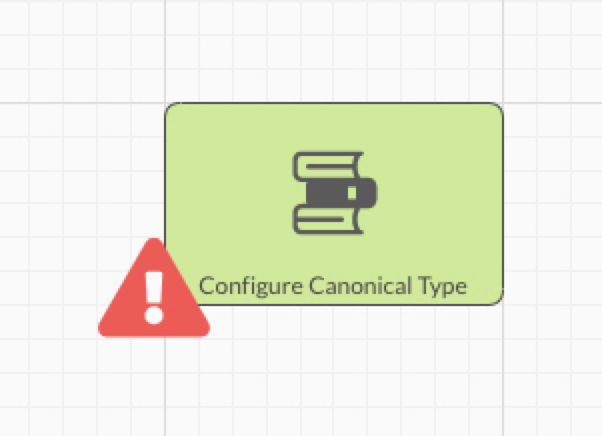
Figure 9.46 An example of a “Canonical Type”-component with a verification error

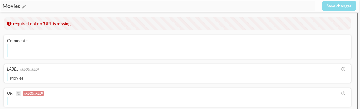
Figure 9.47 A more detailed verification error showns up in the “Canonical Type”-component itself

Dependency analysis

Some additional features become available after performing a verification run. Open your “Canonical Type”-component and click on “ movies” under Known predicates and click on the next to “movie:genre_label.lit”.

Doing so shows the “Dependency Analysis” screen where you can trace back the predicates used to form “movie:genre_label.lit”. Looking at Figure 9.48, you can see that “genres.lit” is imported from a CSV in the movies-class and used in a “Transform Literals” to create “genres_split.lit”. “genres_split.lit” is then used to create a link between movies and genres, creating “genre_link.fwd” in the process. Finally “genre_link.fwd” is called upon in the “Infer by Relationship” between movies and genres. You can request a dependency analysis from every component that takes predicates as input. Remember that Known predicates only shows the predicates that are coming in as input for that component. Predicate statistics, instead, show you predicates that are generated by that component itself.

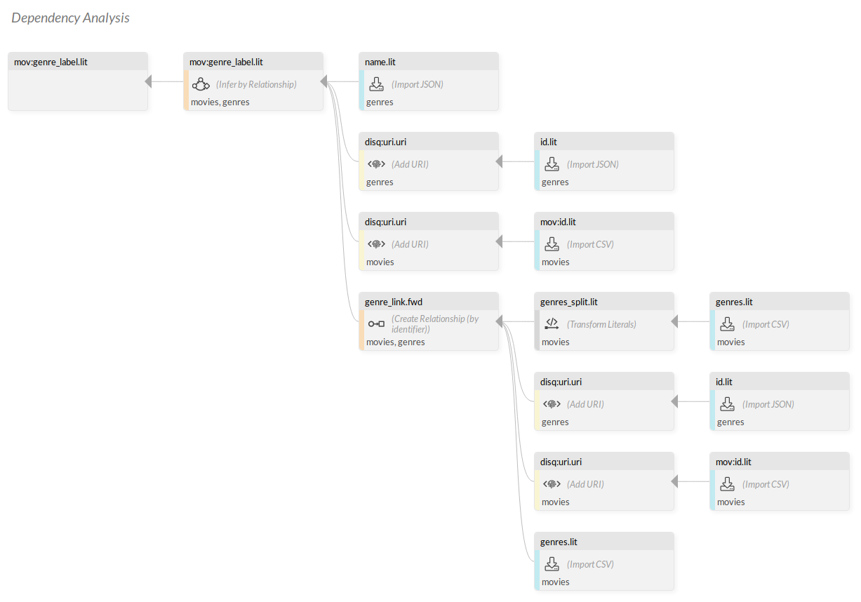
Figure 9.48 Dependency Analysis of “movie:genre_label.lit”, showing the flow of all predicates required to create it

Alternatively, if you know the name of a predicate, but not in which components you might find it, you can click after a verification run to open a dropdown menu (Figure 9.49).

Figure 9.49 The verification dropdown menu, available after a verification run

Aside from re-running the verification, you can select “Analyse dependencies” and fill in any predicate, for example “movie:genre_label.lit”. Doing so brings you to the same “Dependency Analysis” screen as earlier, without having to look a specific component first.

Additionally, if you want to find any components which take specific predicates as input, you can click “Find components that have a predicate as input”. If you have been following this guide, searching for “movie:genre_label.lit” here does not give any results, as you have yet to add it as a facet and property of your canonical type. Searching for “movie:original_title.lit”, however, highlights the “Canonical Type”-component, since it is used here in one of the properties (Figure 9.50).

Figure 9.50 The message-box depicting in how many components “movie:original_title.lit” is used, with “Configure Canonical Type” highlighted in the background

Clicking “Find components that produce a predicate as output”, instead shows you which components produce a specific predicate. For example, searching for “genre_link” here highlights the “Create Relationship”-component (Figure 9.51).

Figure 9.51 The message-box depicting in how many components “genre_link” is created, with “Create Relationship (by identifier)” highlighted in the background

Note

When searching for predicates, input predicates always have to be written with a .lit, while output predicates have to be written without it.

Show execution information

Once you have clicked on and your pipeline is running, you can open the “Pipeline execution log” by pressing the -button. The log shows you the pipelines run-status, which component it is currently executing and the date, time, and run-length of each component. It also shows an error message next to any component which failed to run correctly.

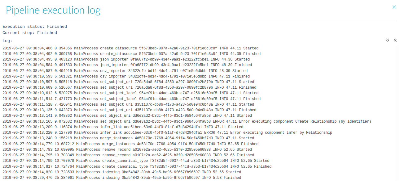
Figure 9.52 The “Pipeline execution log” showing a finished run with an error message in two components

Show execution report

For a more in-depth perspective on your runs, click to open the “DISQOVER Data Ingestion Report”. Here you can find more specific run information, such as:

• the number of warnings and errors encountered while running
• the parameters for your latest run
• timestamps and run length for the entire pipeline
• a timetable, graphically showcasing the timestamps and run length of each component
• the exact error- and warning messages along with their corresponding component
• timestamps for all imported data sources and created canonical types

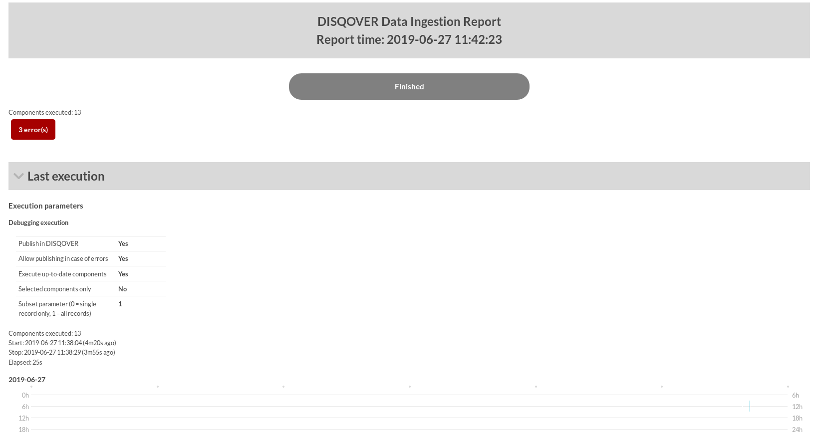
Figure 9.53 The “DISQOVER Data Ingestion Report” showing a finished run with 3 error messages

Fetch resource data

After an initial run, it becomes possible to view the contents of your predicates and resources. This comes in handy when a specific instance does not turn out the way you expected it to, allowing you to check whether its values match up to the requirements of your “Transform Literals” for example.

To do so, click the “Debug tools”-button () to open the dropdown menu (Figure 9.54).

Figure 9.54 The “Debug tools” menu

Fetch resource data

Clicking “Fetch resource data” brings you to its request form. You can fill in these options yourself or, alternatively, you can open one of your components (e.g., your “Import CSV”-component) and click the next to one of your classes on the right. This brings you directly to the “Fetch resource data” request form with all the fields already filled in with the information coming from that component (Figure 9.55).

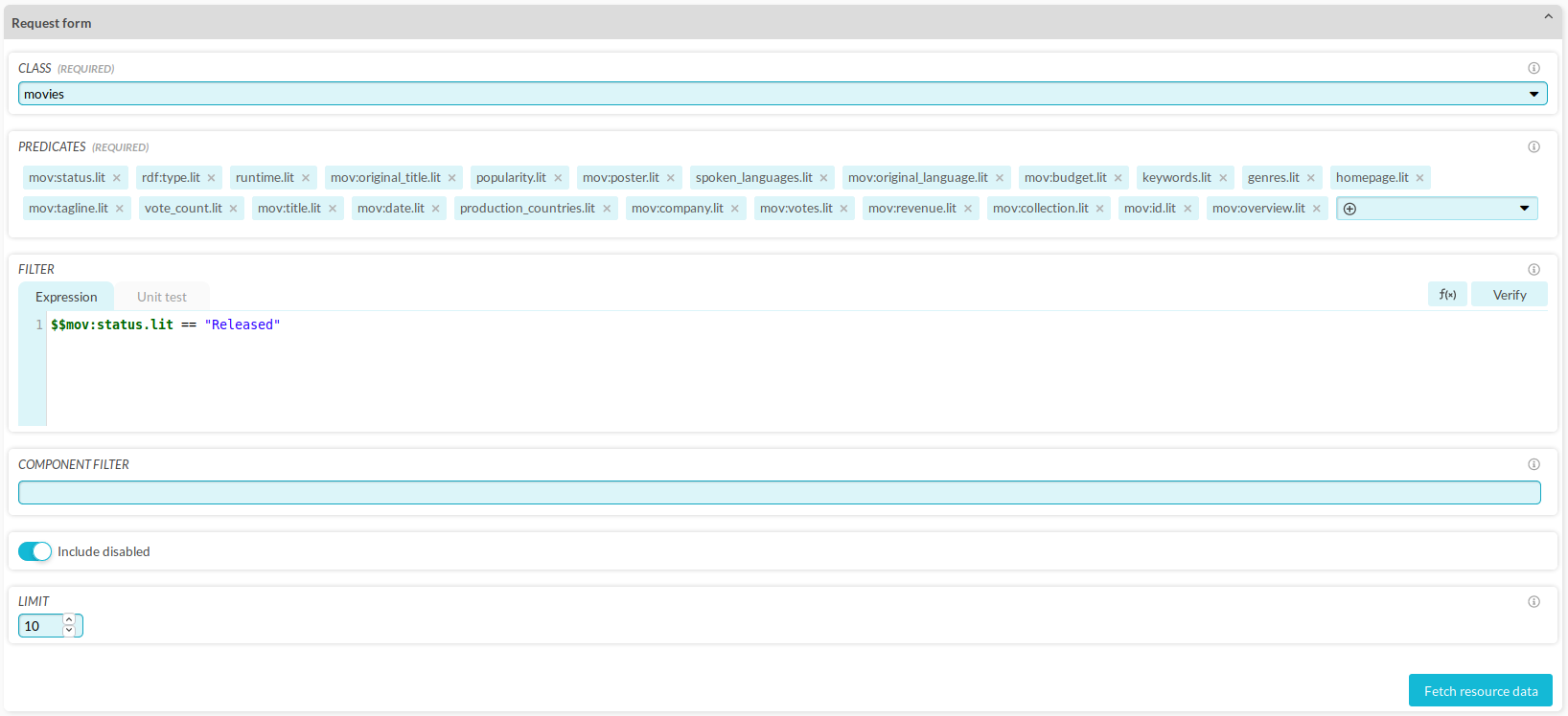
Figure 9.55 The “Fetch resource data” request form, filled in according to the “Import CSV” configuration, looking only for released movies

You receive a table of results, with each row being a separate resource. Clicking on one of these rows opens a detailed depiction of the values of that resource in a JSON-format (Figure 9.56).

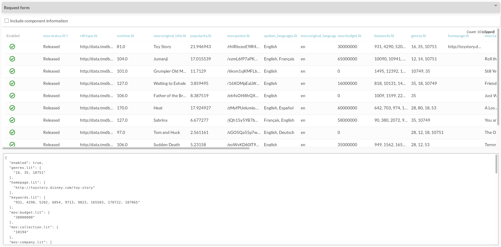
Figure 9.56 The results of the previous “Fetch resource data” request form. The contents of the first resource are being displayed at the bottom in JSON-format

Find URI

Pressing “Find URI” allows you to find resources based on their given URI (“disq:uri.uri”). In the request form, type:

URI	http://data.tmdbexample.com/movie/105045
CLASS	movies
Predicates	movie:title.lit

This shows you that there are three resources in the movies-class with that URI, only one of which is enabled. This is one of the duplicate instances from earlier (Merge Within Class). The first two resources are the original resources coming from the file and end up being disabled upon merging into a single resource, the third one. You also get to see the title of each movie, since you specified “movie:title.lit” as a predicate to find.

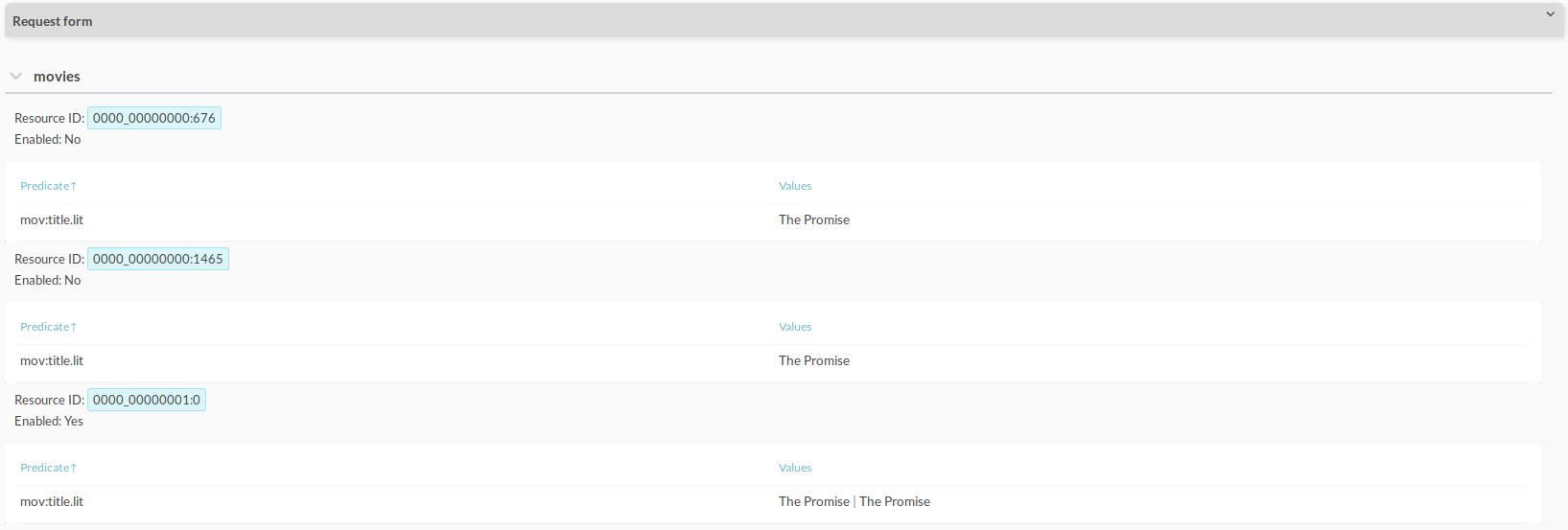
Figure 9.57 The results of a “Find URI”-request, showing all resources which have “http://data.tmdbexample.com/movie/105045” as a URI

Clicking on one of the resource IDs, such as “0000_00000001:0”, automatically takes you to the next section.

Find resources

This is the last tool in “Fetch resource data” and allows you to find resources by their corresponding resource IDs. Run the request with the following options:

Resource IDs	0000_00000001:0
CLASS	movies
Predicates	movie:title.lit

Once again, you see the enabled, merged resource that contains two titles.

Figure 9.58 The results of a “Find resources”-request show the contents of “movie:title.lit” for resource “0000_00000001:0”

9.3.9. Using Remote Data Subscription

As described in section 9.1.2, you can use Remote Data Subscription to subscribe to data from another DISQOVER installation, which is then automatically retrieved. The DISQOVER installation that publishes the data is called a Publisher, the installation that retrieves the data is the Subscriber.

In this example, you configure and use RDS. The Publisher is a DISQOVER installation that contains the movies pipeline that was created in the previous sections and that publishes the “Movie” canonical type. The Subscriber is another DISQOVER installation that subscribes to the Publisher, imports the prepared “Movie” data and ingests it in a different pipeline.

Configuring the Publisher

The Publisher defines which canonical types are available for RDS. A canonical type that is published to RDS, is called a data set. The configuration of the Publisher for RDS takes place within the Data Ingestion Engine and consists of two steps.

1. Specify which canonical types should be turned into data sets. To make a canonical type (in this case: “Movie”) available for RDS, go to the corresponding Configure Canonical Type component, and turn on the option Publish for RDS.
2. Enable “Publish for RDS” in the “Execute Pipeline” dialog.

Figure 9.59 Setting required to publish a canonical type to RDS.

Once the pipeline has run with those settings, the selected canonical types are published and are available to Subscribers. You can verify your published data sets from the “Remote Data Subscription” page, which is accessible from the main menu (). The section “Published Data Sets” contains an overview of your data sets that are available to Subscribers. If you click on the info button of an individual data set, you can see its predicates.

Configuring the Subscriber

The Subscriber subscribes to one or more Publishers and can schedule the timing of data retrieval. The retrieved data then becomes available for use in the Data Ingestion Engine.

Subscribe to a Publisher

You can configure Publishers from the “Remote Data Subscription” page (Figure 9.60), which is accessible from the main menu (). To configure a Publisher, you click “Subscribe to Publisher”.

Figure 9.60 The Remote Data Subscription tab.

A pop-up opens that lets you configure a Publisher. You need to fill in the following options:

• Name: the chosen display name of the Publisher.
• URL: the link to the publisher.
• Username: the username that is used to access the publisher.
• Password: the password of the user that accesses the publisher.

To check if the Subscriber can successfully log in to the new Publisher, you can click “Test Connection”.

Figure 9.61 Subscribing to a Publisher.

Once you have saved the new Publisher configuration, you can see the available canonical types and the scheduled data retrievals.

First you need to select the data sets in which you are interested. Only the selected data sets are retrieved.

To edit the schedule, click the pencil icon (). A new schedule requires some input:

• A display name for the schedule
• The frequency of the data retrieval
• The type of data retrieval. A full retrieval first removes the data from any previous retrievals, while an incremental retrieval only affects data that has changed.

It is possible to add multiple schedules, for example a daily incremental retrieval and a weekly full retrieval.

You can also manually trigger a schedule, so data retrieval happens instantly instead of at the scheduled time.

Import the data

When data from a Publisher has been retrieved, you can import it in the Data Ingestion Engine. To do so, you need to add a “Import Remote Data Source” component. This component type does not have any preceding components.

In this component, you fill in the following options:

• Server: the name of the Publisher.
• Remote Data Set: the name of the canonical type of the Publisher that you want to import
• Class: the name of the class in which the imported data is stored.

When this component runs, all resources and predicates in the retrieved canonical type in the Publisher are automatically imported to in the pipeline. For example, when importing the movies data, the predicates movie:original_title.lit and movie:genre_label are imported in the pipeline.

The following information about the data set is imported:

• Instances in the data set become resources in the class.
• Properties and facets of the data set become predicates of the classes.
• Links to other retrieved data sets from the same Publisher are stored as .rev or .fwd predicates.

Ingest the data

After the import, the retrieved data can be ingested in the pipeline as with any other data. For example, you could link the imported movies to other data sets that are present on the Subscriber.

Configure Canonical Types

If you want to show the predicates in the imported remote data set as properties and facets in DISQOVER, you can easily transfer the original configuration of the remote data set on the Publisher to the Subscriber server.

To do so, open the Configure Canonical Type of the canonical type that contains the remote data set.

Use the scanner () in the Configure Canonical Type component to automatically fill in the options of the canonical type. You need to fill in the following options:

• Publisher identifier: the name of the Publisher.
• Data Set: the name of the Data Set.
• Class: the name of the that contains the remote data.

After running the scanner, the options for facets and properties are automatically copied to the new canonical type.

However, the scanner only works in case the imported class and predicates have not changed. If the predicates were inferred or changed, those properties and facets need to be configured manually.

Configure Typed links

If you created Configure Canonical Type components containing classes that were imported from RDS, you can use the scanner on the Configure Typed Link component to automatically detect and transfer the the configuration of the typed links on the publisher to your pipeline.

To do so, create a Configure Typed Link component, and click on the scanner button ().

You need to fill in the following options:

• Publisher identifier: the name of the publisher.
• Typed link: the typed link between two canonical types you want to recreate.

After running the scanner, the options and relation types for the typed link are automatically copied.

Note that before you can use the scan functionality of the Configure Typed Link component, all the relevant Import Remote Data Set and Configure Typed Link components should exist in the pipeline.

Figure 9.62 A minimal pipeline that ingests remote data

9.3.10. Using Federation

As described in section 9.1.2, you can use Federation to enrich a customer DISQOVER installation with public domain data provided by ONTOFORCE. Federation can be used parallel with RDS.

In this example, you configure and use Federation to enrich the movies pipeline that was created in the previous sections with ONTOFORCE’s canonical types. In addition, you create a link between your own “Movie” canonical type and ONTOFORCE’s “Location” canonical type, and add a new property to the countries instances within “Location”, containing the names of movies produced in those countries.

Enabling Federation

To enable Federation, you need to have access to the System Settings Panel in the Admin Console (Figure 9.63). There, you can fill in the necessary settings to connect to an ONTOFORCE server. The login details for your installation are provided by ONTOFORCE.

Figure 9.63 The settings to enable Federation.

Once federation is enabled, the public canonical types are available on your DISQOVER installation and co-exist with your previously created “Movie” canonical type. For example, whey you search for “clownfish”, you see a hit in your own canonical type “Movie” (because of “Finding Nemo”, for example) and a hit in “Organism” (because of the fish Amphiprion percula).

At this point, there are no links between instances in “Movie” and any of the ONTOFORCE instances. To link your own instances to ONTOFORCE instances, or to add your own properties to existing instances, you need to make pipeline configurations.

Configuring the pipeline

You can now adapt the pipeline to link movies (your data) to their production countries (public data). You also add the movies that were produced in a country as a property to the countries instances. This requires two new pipeline components, as shown in Figure 9.64.

Figure 9.64 The pipeline components needed for Federation.

Prerequisites

The public data contains a canonical type Location in which some instances are countries. The URIs of those instances are of the form http://ns.ontoforce.com/datasets/countries/US.

The movies database contains a predicate production_countries_split.lit. You first need to extract this predicate into a separate class production_countries (using a “Extract Class (distinct)”-component), in which the resources are individual countries that have the same URI as the countries in the public data. The relationship between production_countries and movies is called produced_in_country.rev.

In the following steps, you can then federate this class to the public Location class.

Federating

To start federating, you add a “Synchronize Federated Class”-component to the pipeline. You fill in the following options:

Option	Value
Class	production_countries
MATCH URI PREDICATE	disq:uri.uri

Important

This is a simple example of Federation, in which you can use an already single valued URI for URI matching. For more information on Federation, see Synchronize Federated Class.

Configuring the federated canonical type

After federating, you need to configure the federated canonical type using a “Configure Canonical Type”-component. For this, you need to use the URI of ONTOFORCE’s canonical type. See section 6.3 and Configure Canonical Type for more details on the URIs and icons, respectively.

In this case, you can fill in the following information:

Option	Value
Label	Production Country
URI	http://ns.ontoforce.com/ontologies/integration_ontology#Location
Icon	font-awesome fa-globe
Classes	production_countries

To add a property to “Production Country” that contains the names of the movies produced in that country, go to Properties/Facets and add:

Option	Value
Label	Movies produced in the country
URI	http://config.tmdbexample.com/ontologies/movies/properties/produced_in_the_country
Predicates	produced_in_country.rev

End result

After running the pipeline with federation enabled and the newly configured “Country” canonical type, all local and public canonical types are available for searching.